Dear Reader

I have been working on a multithreaded implementation of the Backpropagation algorithm. The most computationally intensive parts of a learning iteration are the forward-propagation and the backpropagation steps which are used in all algorithms to determine the gradients. The main difference between these algorithms is how these gradients are used to update the network:

• In simple Backpropagation a weighted sum of the previous and the current gradients is used to update the weights, the current weights are multiplied by a momentum value (0.5 < m < 1.0) and the previous weights are multiplied by (1.0 – m).  In the online version of the algorithms the weights are updated after each data sample is processed.
• The Batch Backpropagation is also using a weighted sum of the previous and the current gradients, but it is only updating the weights after a certain amount of data samples are processed to find a common gradient. Then this gradient is used to update the network. The batch size can be an arbitrarily chosen number depending on the task, or the whole dataset.
• The Resilient Propagation algorithm is using a sub-algorithm to determine the weight updates and it only takes into account the sign of the gradient values. It is a batch algorithm that only updates the weights after the whole dataset is processed.

If data oriented task distribution is the base of our parallelisation then only batch algorithms can be considered, and only those that update weights after the whole dataset is processed. My first implementation for distributed processing is the Batch Backpropagation algorithm.

At first it finds out the number of possible concurrent threads on the current architecture. Then it creates the same amount of neural network models by copying the neural network it was initialised with. These networks will share pointers to the actual data.

auto concurentThreadsSupported = thread::hardware_concurrency();
if (distributedNeuralNetworks->size() == 0)
{
	for (uint i = 0; i < concurentThreadsSupported; ++i) 	{ 		(*distributedNeuralNetworks).push_back( 			make_shared( 				CNeuralNetwork(*NeuralNetwork->Parameters)));
	}
}

Then it creates the same amount of std::future asynchronous tasks. These tasks are going to run parallel each using a separate neural network model to avoid concurrency issues. Each parallel task contains a forward propagation and a backpropagation step, but executed only on part of the data. These tasks are going to run in parallel, each on their own dedicated CPU.

auto inputDataCount = NN.InputData->GetColumns();
auto BatchPosition = 0u;
auto BatchEndPosition = 0u;
auto BatchSize = inputDataCount / concurentThreadsSupported + 1;
unique_ptr tasks =
	make_unique(vector());
uint distributionIndex = 0;
while (BatchPosition = inputDataCount)
	{
		BatchPosition = 0;
	}
	BatchEndPosition = BatchPosition + BatchSize;
	if (BatchEndPosition > inputDataCount)
	{
		BatchEndPosition = inputDataCount;
	}

	future calculate(
		async([this](uint start, uint end, uint index)
	{
		return CalculateGradients(start, end, index);
	},
	BatchPosition, BatchEndPosition, distributionIndex));
	tasks->push_back(move(calculate));

	BatchPosition = BatchEndPosition;
	distributionIndex++;
}

Once these tasks are finished we have to summarize their results and update our original neural network with these new parameters. The gradients can be simply added together.

UpdateWeights();

for (auto &d : (*distributedNeuralNetworks))
{
	d->NeuronOutputs[0] = NN.NeuronOutputs[0];
	for (uint layer = 1; layer Weight[layer] = NN.Weight[layer];
		d->Bias[layer] = NN.Bias[layer];
		d->PreviousWeightGradient[layer] = d->WeightGradient[layer];
		d->PreviousBiasGradient[layer] = d->BiasGradient[layer];
		d->NeuronOutputs[layer] = NN.NeuronOutputs[layer];
		d->WeightGradient[layer] = 0.0;
		d->BiasGradient[layer] = 0.0;
	}
}

However, at this point we are still missing an important bit which is the current output of our neural network. To get these values we have to execute a forward-propagation step on the network with the newly determined Weight and Bias values. This is computationally intensive, it involves matrix product calculations, so this can be run again in parallel.

BatchPosition = 0u;
BatchEndPosition = 0u;
BatchSize = inputDataCount / concurentThreadsSupported + 1;

unique_ptr post_tasks =
	make_unique(vector());
distributionIndex = 0;
while (BatchPosition = inputDataCount)
	{
		BatchPosition = 0;
	}
	BatchEndPosition = BatchPosition + BatchSize;
	if (BatchEndPosition > inputDataCount)
	{
		BatchEndPosition = inputDataCount;
	}

	future post_calculate(async([this](uint start, uint end, uint index)
	{
		CNeuralNetwork &nn = (*(*distributedNeuralNetworks)[index]);
		for (auto VectorIndex = start; VectorIndex GetColumn(VectorIndex);
			*nn.Target = nn.TargetData->GetColumn(VectorIndex);
			PropagateForward(nn);
			{
				Lock lock(*locker);
				NN.OutputData->SetColumn(*nn.Output, VectorIndex);
			}
		}
	}, BatchPosition, BatchEndPosition, distributionIndex));
	post_tasks->push_back(move(post_calculate));

	BatchPosition = BatchEndPosition;
	distributionIndex++;
}

for (auto &e : *post_tasks)
{
	e.get();
}

(Ok, at this point I have decided that I am going to move away from wordpress.com. Can’t insert code snippets easily unless I install a plugin – but that would cost me £200 a year, because only business users can use plugins. I am doing this stuff in my free time and I am not getting paid for it. I’ve been trying to avoid messing with website designs up until now, but it seems there is no other way.)

The result is much faster processing. In the case of the Distributed Resilient Propagation algorithm the convergence became so quick on 8 parallel hardware threads that the network can reach a fully trained state within seconds. The Batch Backpropagation algorithm has a much slower convergence but it is still useful for different types of data/tasks.

Here are some speed measurement values in kCPS, which is 1000 neural connections processed within a second, measured on a 4GHz Intel Core i7 processor with 8 hardware threads:

• Backpropagation: 8200 kCPS, fully trained … well, whenever, maybe after 8000 or 10000 iterations, but it keeps converging even after that. This is not really an efficient algorithm to be honest.
• Batch Backpropagation: 8500 kCPS, and it has a slightly better convergence than the non-batch version, I would say after 5000 iterations it is already in a much better state then the non-batch after 10000.
• Resilient Propagation: 11700 kCPS, and it is well-trained after 500 iterations already, but it still converges quite well until it reaches 1500 iterations.
• Distributed Batch Backpropagation: 27200 kCPS, and it is fairly well trained after 5000 iterations. Around 5000 iterations (this number probably depends on the preconditioning of the network too) it starts oscillating in the error, probably because of the way the weights are updated. I still have to investigate whether this is a feature or a bug.
• Distributed Resilient Propagation: 27900 kCPS, fully trained after 1500 iterations.

Of course it is very relative what one should consider to be a fully trained network, and the above numbers will be different for other types of tasks. For very large and complex data sets the number of necessary iterations could be higher. Anyhow, for this testing task that is making the network learn power functions like parabolas and the root function these numbers of iterations were enough.

I have access to a computer with 40 hardware threads, I will update this post if I get a chance to test my algorithms on it.

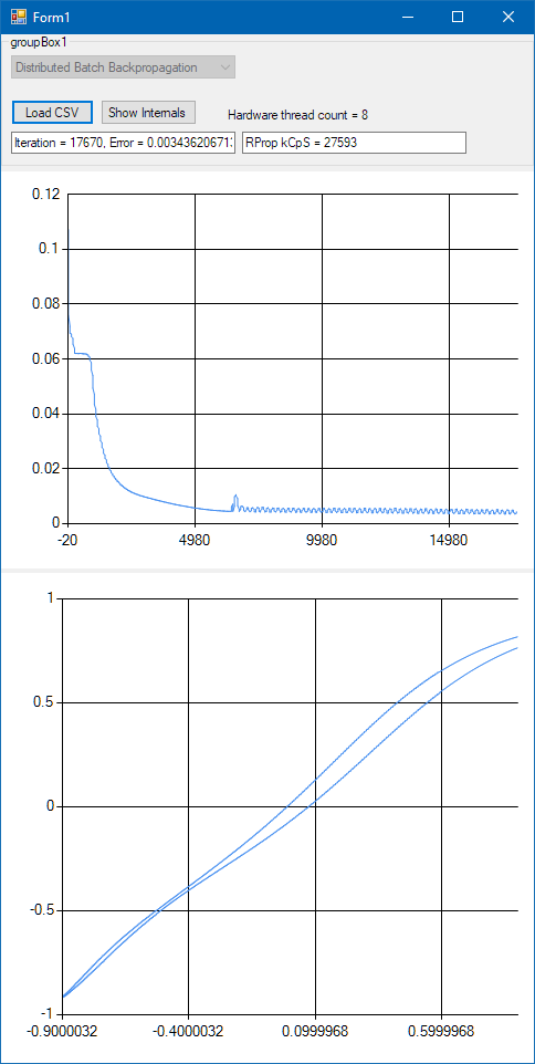
Oscillations in the error in the case of the Distributed Batch Backpropagation algorithm

Update: I had a chance to test the algorithms on a 3GHz dual-Xeon 20 core PC which has 40 harware threads. When I was using 30 threads, the Distributed Resilient Propagation algorithm easily reached 55000 kCPS, but with 40 hardware threads this number was only 45000 kCPS. I guess this is down to the fact that every iteration must also contain a single-threaded operation, and the data set I was testing with is just not large enough to give enough work to 40 threads. I will retest it with a larger data set soon.

Update 2: In the meantime I managed to improve the parallel processing part of the algorithms, got rid of the final parallel bit that was doing an extra forward-propagation step and filling in the output vectors. I have moved the part that is changing the global output vector under the first parallel processing code. Now the Distributed Resilient Propagation algorithm easily reaches 41500 kCPS on my 4GHz core i7 using 8 hardware threads.

Update 3: A further improvement I made was to change how the neural networks are copied under the hood. Instead of creating new networks for distributed processing I made use of my copy constructors to create new network instances. The copy constructor is not creating a copy of every network parameter though, it shares those that remain the same for all networks during parallel processing.  Since the Matrix class is thread-safe already I didn’t even have to worry about concurrency issues during calculations. This reduced the time the algorithm takes with copying values from and to the global model, and it also reduced the time it took to create all the copies of the networks. Now initialisation happens almost instantly. On my 8 core PC the Distributed Resilient Propagation algorithm reached 43200 kCPS, and on the 40 core Xeon PC it reached 69000 kCPS – a new record, I haven’t seen this high number before!

To the left: Core i7 4GHz, 4 cores, 8 hardware threads. To the right: Dual Xeon 3GHz, 20 cores, 40 hardware threads.

 

Update 4: I have made some tests with a different, much larger data set we used in a past project. It has 13 inputs and 8 outputs, it has 30000 samples, and the neural network being trained with it has one hidden layer only with 100 neurons. That is 1300 + 800 = 2100 neural connections. The core i7 with 8 hardware threads reached a processing speed of 150000 kCPS (that is 150 million neural connections processed per second!), and the dual Xeon PC with 40 hardware threads reached 468000 kCPS! (which is 468 million neural connections processed per second). These numbers truly compare the real processing power of these computers and they show that the algorithm makes full use of the power of parallel processing. The core i7 utilised 4687 kCPS/GHz/core, the Xeon utilised 3900 kCPS/GHz/core. It seems it’s time for me to start using the unit MCpS.
468 MCpS is almost a half GCpS! 🙂