This post will try to give you a brief introduction to artificial neural networks or at least to some types of them. I will skip the introduction to biological neural networks as I am neither a biologist nor a doctor, I prefer not to write about what I do not fully understand.

Overview of artificial neural networks and supervised learning
I think it is very important to note that artificial neural networks are neither magical AI circuits nor oracles with the ability of predicting stock market movements. You can save one as a file on the disk and you can name it skynet if you like but it will not get more intelligent from that. In reality they are simply mathematical tools that can come very handy in solving certain problems (and can prove to be completely useless for others).
It is best to imagine a neural network as a black box. This black box has inputs and outputs. In an uninitialized state this box will have a completely undefined behaviour: it will give arbitrary answers to any inputs (although it will always give the same answers to the same inputs). Imagine this inital state of the box as one with the highest disorder (or entropy), no effort has yet been made to make it do what we expect it to do. This state can be analogous with the brain of a newborn baby – he or she is just about to start experiencing the whole world.
There is a process called supervised learning during which the box is fed with input-output patterns and its internal entropy is reduced by making it learn the relationships between these inputs and outputs. There is another word for this process in mathematics: regression analysis, and neural networks are not trying to be anything more than that either. The only thing that makes artificial neural networks unique is that the applied mathematical function used for modelling is based on how we think the brain works.
The learning process starts by feeding our inputs to the uninitialized box and comparing the desired outputs with the actual ones. At first we will most likely receive a big difference as the box have no idea about the desired IO relationships. This difference is called the error of the neural network. During the training process our aim is to minimize this error as much as possible by iteratively feeding the same IO patterns to it again and again, and making such adjustments to the internal state of the box so that its overall error (or entropy) will decrease.
Inside the box – the neuron
The atomic mathematical building blocks of neural networks are called neurons. They are similar to biological neurons in that they give outputs to inputs and they have persisting properties (weights), which means that they are able to adjust and store internal states that influence their outputs. (I personally prefer the analogy with transistors more than with braincells. Human braincells are far more complex than the mathematical neuron, they are almost little computers themselves.)
The inputs arriving to a neuron are all normalized by being multiplied by a weight value. This weight can be imagined as priority or importance levels added to each input. Then the weighted input values are summarized. After this an activation function f is applied to the weighted sum.
\[y_i = f(net_i) = f\left(\sum\limits_{j} w_{i j} y_j \right)\]

Activation functions
In order to train the neural network (and its neurons of course) we need to determine the difference between the actual output values of the neuron and the desired output values. This difference also forms a function that is called error function. The error function is a surface in n dimensional space and it has a global minimum point. The training process aims to find this minimum point so first it needs to find the steepness of the surface. The steepness is the best direction (or at least the best guess) towards the global minumum.
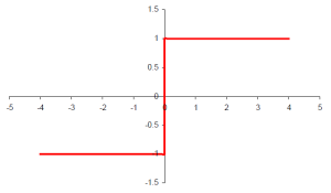
This error surface will depend on the linear combination of the activation functions. The gradient of this surface can only be determined at any point in an interval if the activation function itself is continuous and differentiable at least once in that interval. If we want to model the behavior of the biological neuron we could use the step or signum activation functions. The behaviour we get from these functions is that the neuron will only output values (or in other words it will only fire) if the summarized inputs reach a certain value.
\[y_i =sign(x)\]
The signum activation function
Although the above activation functions are continuous unfortunately their linear combination is not. By reducing the 90 degree steepness of this function it can be made continuous though. A very popular activation function does just this: the sigmoid or logistic distribution function. This is a real function on the (0,1) interval:
\[s_c:R\Rightarrow (0,1) \ \ \ s_c (x)=\frac{1}{1+e^{-cx}}.\]
 The sigmoid activation function (shapes are for c=1, c=2 and c=3 values)
The sigmoid function uses a c constant that determines the steepness of the activation function. This c value is chosen when preconditioning the network and it is not updated during the training process. It is a global property for the whole neural network (all neurons use the same steepness). By increasing the c value the sigmoid function converges to the step function.
We need the derivative of the sigmoid function to determine the gradient of the error surface:
\[\frac{d}{dx} s(x)= \frac{e^{-x}}{(1+e^{-x})^2}=s(x)(1-s(x)).\]
An alternative to the sigmoid function is the symmetrical sigmoid, which is the hyperbolic tangent of the x/2 value.
\[S(x)=2s(x)-1=\frac{1-e{-x}}{1+e{-x}}=tanh \frac{x}{2}.\]
\[\frac{d}{dx} S(x)= \frac{e^{-x} \left(1+e^{-x}\right) + e^{-x} \left(1-e^{-x}\right)}{\left(1+e^{-x}\right)^2}=\frac {2e^{-x}}{\left(1+e^{-x}\right)^2}=\frac{1}{2} \left(1-S^2 (x)\right).\]
The symmetrical sigmoid activation function and its derivative.


