Dear Reader,

I decided to publish an old version of the RProp algorithm I wrote back in 2003 that demonstrates how the algorithm modified to use matrix algebra works.

The demo can be downloaded from here, both source files and binaries:

https://github.com/bulyaki/NeuralNetworkTrainer

Originally this version was lacking a couple of libraries and I could not start it at all on my Windows PC. I have rebuilt it and made some changes to the project configuration so that it linked all necessary VCL libraries to the EXE. Right now it works perfectly on Windows 10 (and probably on all Windows OSs back to Windows XP) without installing any extra prerequisites.

It took me some time to be able to build it again, here are the prerequisites in case you would like to build it too:

• Borland C++ Builder 6
• Windows SDK – mainly because of the OpenGL libraries

After installing the Windows SDK you may need to take some extra steps so that C++ Builder could import some required libraries. To do this open a command prompt and navigate to your $(bcb)\lib folder. Here you will need to use the following commands:

implib opengl32.lib c:\windows\system\opengl32.dll
implib glu32.lib c:\windows\system\glu32.dll
implib winmm.lib c:\windows\system\winmm.dll

For me these were the only library dependencies I needed to convert to Borland format.

Here is how to use the application itself:

First you have to click on the “Load CSV Data” menu item or toolbar button. For this purpose you need a CSV file that contains both the inputs and the desired targets (training patterns) for the Neural Network.

Each column is either an input vector or an output vector, inputs come first, outputs afterwards. So they should look something like this (this is a snippet from the sqr_sqrt_1500_rows.csv file contained in the repository):

-75,5625,-421875,31640625,-2373046875,8.660254038
-74.9,5610.01,-420189.749,31472212.2,-2357268694,8.654478609
-74.8,5595.04,-418508.992,31304472.6,-2341574551,8.648699324
-74.7,5580.09,-416832.723,31137404.41,-2325964109,8.642916175
-74.6,5565.16,-415160.936,30971005.83,-2310437035,8.637129153
-74.5,5550.25,-413493.625,30805275.06,-2294992992,8.631338251
-74.4,5535.36,-411830.784,30640210.33,-2279631649,8.625543461
-74.3,5520.49,-410172.407,30475809.84,-2264352671,8.619744776
-74.2,5505.64,-408518.488,30312071.81,-2249155728,8.613942187
-74.1,5490.81,-406869.021,30148994.46,-2234040489,8.608135687
-74,5476,-405224,29986576,-2219006624,8.602325267

The piece of data above has one inputs, and 5 outputs. The inputs are numbers from -75.0 to -74.0 with 0.1 increments. The outputs are second, third, fourth and fifth powers of the inputs, and the last output column is the square root of the input.
Out1 = In^2
Out2 = In^3
Out3 = In^4
Out4 = In^5
Out5 = In^(1/2)

Then you will have to specify how many inputs and outputs you wish to connect to your Neural Network. Click on the Options -> Neural Network Setup menu item.

Now that we know the number of inputs and outputs, you have to specify the dimensions of your neural network. Let’s create a network with two hidden layers, with each layer containing 10 neurons:

We can leave the number of iterations 10000. Then click on the “Start” button (little play button on the toolbar) and the training process begins.

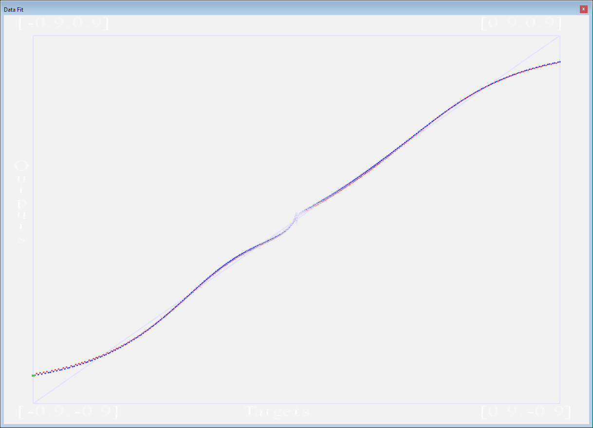
You will see three buttons with graph icons in the Learning Progress window that open some data visualisation dialogs. These dialogs are all using OpenGL. The first button will show you the current regression of the neural networks outputs:

The graph in the middle shows the regression of the output and the training vectors. In the sqr_sqrt_1500_rows.csv file the first output is a parabola function (y=x^2, x=[-75.0 … +75.0]).
On the above photo you can see how both sides of the parabola is taking shape, and eventually it will reach a close to 45 degree straight line (well, more or less). Below are the DataFit windows of the remaining four outputs. What is most interesting is the last output, which is trying to learn a square root function. This function doesn’t have many values around zero, and it is reflected well in the regression below. Individual values that are significantly different from the rest of the training set are taking longer to learn. The blue dots here are outputs of the network from the training set, the red dots are outputs from the test set.

Obviously neural networks should not be used to for functions where we know the connection between input and output variables, but such functions are very useful for testing our network and our algorithm.

The second graph button will show you a graph of the error values, along with the test set (in red). There is a context sensitive toolbar at the bottom of the application which changes its function when a visualisation window is focused. In the case of the Errors window it allows you to change the X and the Y axis zoom.

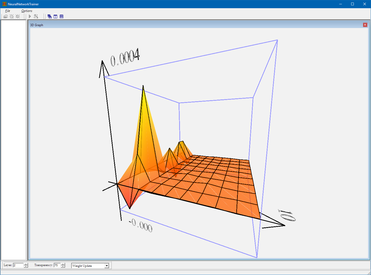
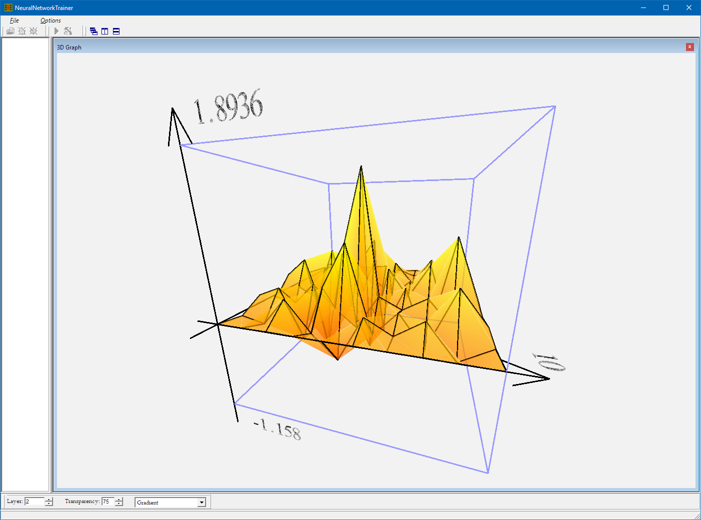
The third data visualisation button opens a 3D graph that shows certain values within the neural network in real time. You can control what parameter in which layers you would like to visualise:

Weights between the first and the second hidden layer:

Weight Updates between the first and the second hidden layer:

Gradients between the first and the second hidden layer:

Meta-Gradient values between the first and the second hidden layer:

Please note that I created the above application about 15 years ago, so the code in the repository is NOT a faithful representation of my current programming and design abilities. Also, if you find bugs in the code you are welcome to fix them yourself, and I will also try to fix any bugs I find later on.

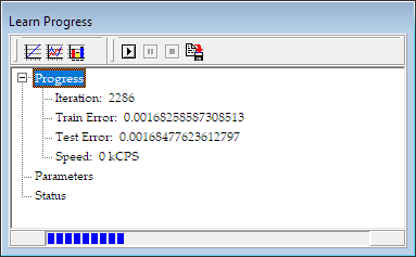
The Learn Progress window shows you a progress bar at the bottom. When all the pre-configured iterations are completed it will open up a save-dialog, and allow you to save the current state of the Neural Network as an NNS (Neural Network State) file. I will leave it to you to figure out the composition of this file from the source code.

The speed of the calculations is measured in kCPS, which is kilo-connections per second. In other words this is the number of neural connections processed within a second, divided by 1000.

The last button on the toolbar of the Learn Progress dialog will allow you to save an NNS file at any point during the training process.

This application does some interesting stuff so that it could display text and numbers in 3D. I created a 3D scene of the whole alphabet with various fonts in 3D Studio Max. Then I exported these objects to 3DS files. From 3DS I was able to use a converter application that created vertex array source code snippets. These snippets are then loaded and normalized inside the application, and saved to .DAT files. The bit of code that created the .DAT files is in TextOutGL.cpp, but it’s commented out as it is only needed once.

Then these .DAT files are loaded, and by using the TTextOutGL::PrintText function I was able to print text to the OpenGL canvas with the fonts of my choice. Please remember that this application was created in 2003, and my options were quite limited at the time for displaying 3D graphics.

I am already working on a C# version of this algorithm which I’m planning to publish in the coming weeks. Also once ready, I plan to republish these blog posts as one long article on CodeProject.